(and a bug that taught me more than the code did)
7/21/2026
Since the last post I got back into VSCode and Qiskit properly, and this update is less about a result and more about a mistake I almost didn’t catch
GETTING THE FIRST NUMBER
The finance module of Qiskit, namely the (qiskit-finance) module, already contains everything you require, including a LogNormalDistribution circuit that encodes the probability distribution of the future price of the underlying asset, and an EuropeanCallPricingObjective circuit that encodes the payoff function into the amplitude of one of its qubits. By combining these components and then passing them through IterativeAmplitudeEstimation, you obtain the price of your option.
As many parts of the API were new to me, I used an AI tool (Manus) to write my first draft of the script, the same way I used AI for debugging and concept clarification in the previous project. It didn’t give any error, came up with the price estimate almost equal to the $10.45 baseline estimated using Black Scholes model, and even showed the ef fect of “qubit gap” which I hoped it would, wherein the estimates are very poor for low qubit numbers but converge to the correct value for higher numbers.
Notable Bug I Encountered
I Ran that exact same script a second time, no changes at all just to confirm the number. Got an entirely different outcome – not even remotely close to the last one so clearly something was wrong
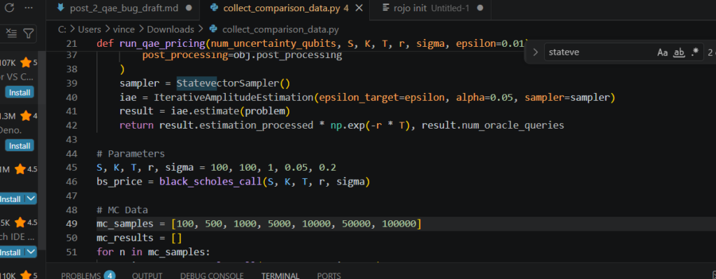
What I discovered was that the culprit in this case was relatively easy to pin down: there wasn’t any seeding in the script. The randomness is entirely regenerated when running each iteration of the classical Monte Carlo simulation as well as the quantum sampling simulation, making a single pass of the qubit numbers simply a random noisy data point. What the original version had generated was essentially a fluke – lucky, unlucky, doesnt matter
This is a sort of continuation of the “1,000 samples landed above 500 samples” issue of the previous post.
Fixing It
This “fix” is the same as the classical baseline idea: do not rely on single runs anymore and use the average results of many repetitions instead. Now for each qubit size, I perform 8 repetitions of the price calculation circuit with different seeds and provide an average error and spread among those repetitions, rather than a single misleading value.
# before — every run draws fresh randomness, nothing is reproducible
sampler = StatevectorSampler(default_shots=4096)

# after — seeded, and repeated across trials instead of trusting one run
sampler = StatevectorSampler(seed=seed, default_shots=4096)
Here’s what that actually looks like after alot of debugging
| Qubits | Average error vs. exact price | Spread across trials |
|---|---|---|
| 2 | $1.43 | ± $0.07 |
| 3 | $0.26 | ± $0.07 |
| 4 | $0.14 | ± $0.05 |
| 5 | $0.12 | ± $0.06 |
| 6 | $0.09 | ± $0.04 |
| 7 | $0.06 | ± $0.06 |
This is the actual implementation of what I was talking about. From 2 qubits to 7 qubits, there’s a reduction of over 20 times in errors, and this time it’s a smooth, monotonically increasing function rather than a one-shot noisy result. I applied the same concepts I learned from the last project on quantum computing
Lesson learned
The real lesson here isn’t about quantum computing at all; it is the lesson of being cautious about accepting an answer when the code works without any errors and gives you a sensible number. Being error-free doesn’t mean being right, and it’s always better to constantly change and improve your methodology to produce the optimal results. I had a similar experience last year when running the code for my EAQEC project, atleast 13 versions of the main code was created.
Next up I want to put the classical Monte Carlo convergence and this QAE convergence on the same chart
Leave a Reply